Use these step by step instructions to sort your lists with maximum efficiency in Excel.

Sorting Lists

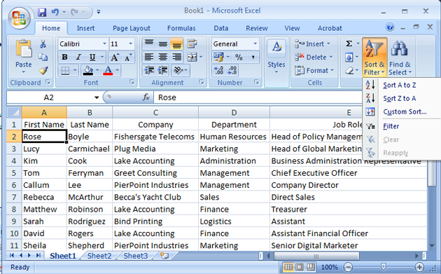
Excel can sort columns into order alphabetically and numerically. You can perform a single column sort of multi column sort.

The Sort command can be found on the Home tab under the Editing group.

Important: When setting up the list, include a set of column headings (as example below). These are used to control the sort columns. The list must be sequential, i.e. no row gaps from the top of the list to bottom.

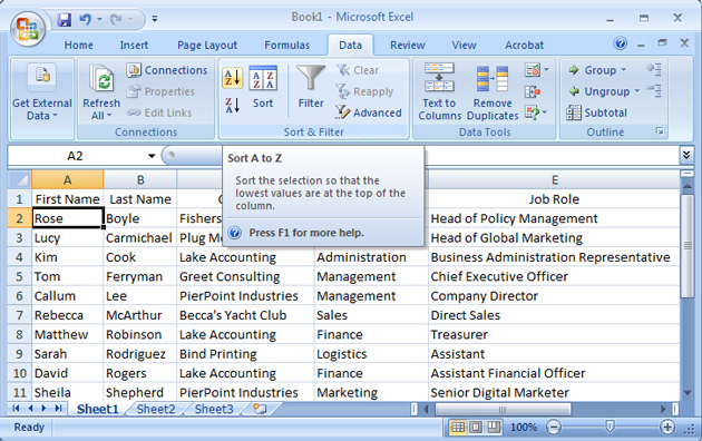
Single Column Sort

Click into a cell in the column that you wish to sort by, as in the example below the First Name column.

Select the Data tab, then to sort by A to Z or Z to A.

You can sort data by text (A to Z or Z to A), numbers (smallest to largest or largest to smallest), and dates and times (oldest to newest and newest to oldest) in one or more columns.

The table is sorted by the selected column.

Note: Data sort can also be found under the Home tab, under the Editing group.

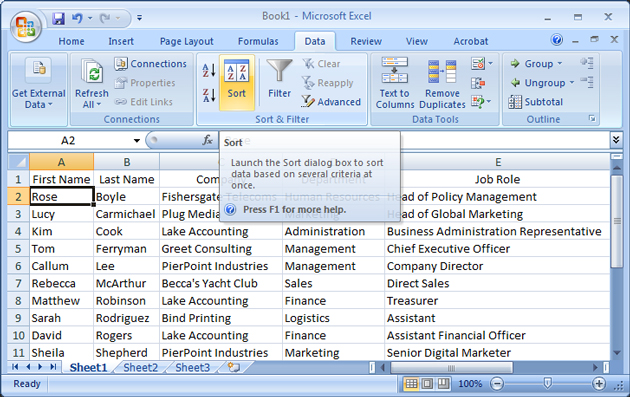
Multi Column Sorting

A list can be sorted by a maximum of 64 columns. In the example below you may wish to sort by Company, then Department, Job Role, Last Name and First Name. A five column sort.

Click in a cell within the table.

Select the Data tab, then click on Sort in the Sort and Filter group.

Select the first Column to sort by from the Sort By box, i.e. Last Name.

Select to Sort On Values.

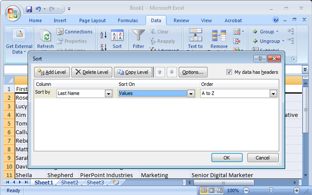
Select the order A to Z or Z to A.

As we are sorting by more than one column we now need to add the further levels.

Select Add Level.

Choose then to Sort By - Department on Values.

Repeat this process until the five sort levels are set.

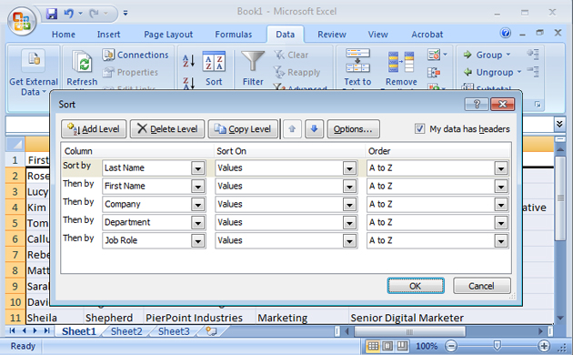
Note: Make sure that the tick is in the box My data has headers, otherwise the headings will be sorted into alphabetical order as well.

Click on OK.

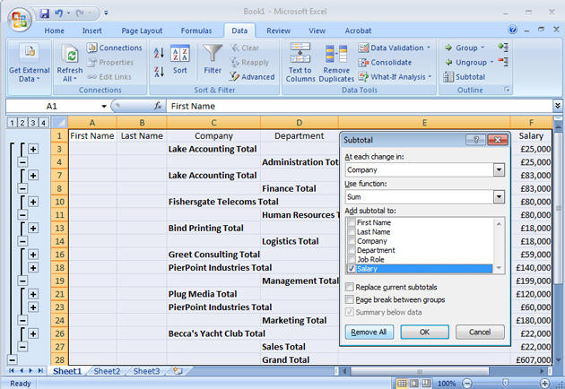
Subtotals

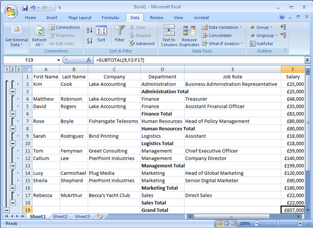
When a list has been sorted into order, it is very easy to ask Excel to subtotal a list for you. Say for instance that you wished to sort by Department and then subtotal the Departmental salaries.

• Sort the list prior to creating subtotals, i.e. by Department
• Click into the table to Subtotal
• Select the Data tab and choose Subtotal
• Select the appropriate field heading in the At each change box - This should be the first column you sorted by, i.e. in the example Department
• Select in the Use function box, the function to apply Sum is the default
• Select in Add subtotal to the column where the subtotals are to be placed, ie. in example Salary
• Select OK

Other Options in the Subtotal Box

Replace Current Subtotals

If further subtotals are required in the same list, de-activate this box. Within a list you could find the sum of salaries and count how many people in the department. To do this change the sum function to count.

Page Break Between Groups

Ensure each subtotalled Group is on a separate page.

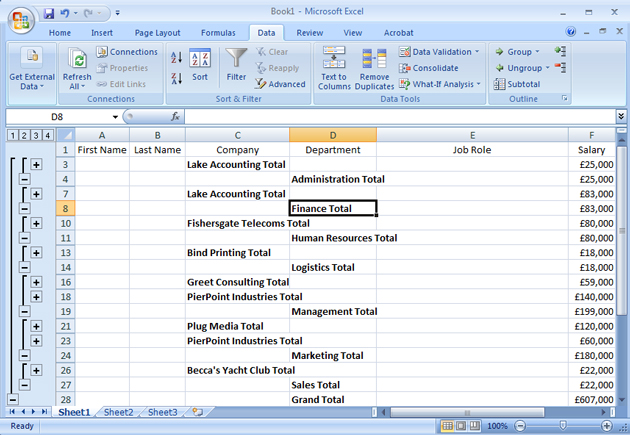
The list is subtotalled. An Outline Format is created; brackets appear on the left hand side of the screen. These can be used to Expand or Collapse the list. In addition at the top left of the screen, buttons appear that enable the list to be Expanded or Collapsed.

You can have multiple subtotals in a list, so you could choose to find average salaries per department. Just make sure you take off Replace current subtotals.

Remove Subtotalling

• Click in the list
• Select the Data menu, then Subtotal
• Click on Removal All

Note: If you have several subtotals, remove all will take all of them away.

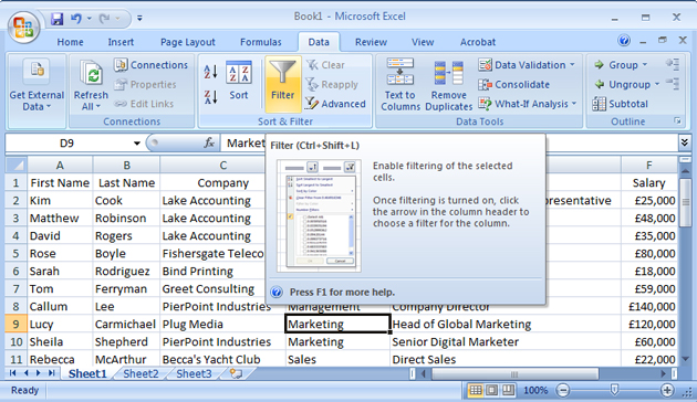
Using Autofilter

Quite often it is necessary to look through a list of information for records meeting a certain criteria, i.e. everybody that works in the Marketing Department, earning over £15,000. It is very easy to extract information from a list (Database) by using Excel's Autofilter. This enables selection from various columns within the database.

• Click within the Database area
• Select the Data tab
• Select Filter from the Sort and Filter group.

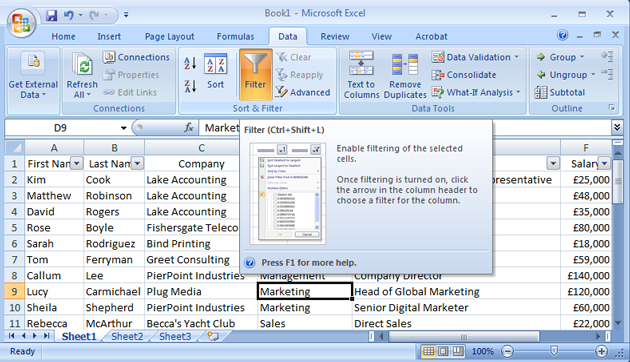
A series of filter arrows are placed alongside the headings. These are used to filter the information.

Objective: To find all personnel working in the marketing department

• Click on the filter arrow to the right of Department
• De-select (Select All)
• Click in the box alongside Marketing to view records for this Department

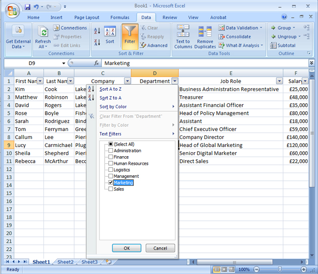
Records that do not match are hidden and only records matching the Marketing Department are displayed.

View All Records

Notice that the filter arrow changes to indicate the column that has been filtered. You will see this symbol on all columns that have been filtered.

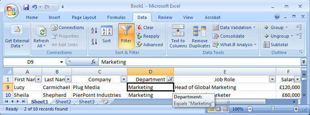
To see all the records select Clear from the Sort and Filter Options, or choose Select all from the filters arrows of the filtered columns.

Different Type of Column Filters

Excel 2010 also provides filters relevant to the type of column. Columns can be made up of text, numbers and dates. Select the filter arrow to the right of the column heading to see the type of filters available.

Removing the Filter

Select the Data tab, click on the Filter button to turn this option off.

Still need help? Why not book yourself onto a Beginners Excel or Advanced Excel training course.